11 Analysis of variance
Throughout this chapter, we will provide a pipeline to help you wrangle data, perform statistical analyses, and (perhaps most importantly) visualize data in R.
Let’s load the usual packages, and one new package called car (Companion to Applied Regression).
library(gapminder)
library(tidyverse)
library(car)  # for Levene's test
11.1 ANOVA in a nutshell
Analysis of variance (ANOVA). ANOVA tells us whether multiple groups are significantly different from each other. We can write our general hypotheses as this:
- H\(_0\): there is no difference between the groups.
- H\(_a\): there is a difference between the groups.
Like how the t-test used the t statistic, ANOVA uses the F statistic. In general:
- A small F means there likely is not a difference between the groups (H0).
- A large F means there likely is a difference between the groups (Ha).
ANOVA assumes that
- All groups have equal variance, and
- All groups have a normal distribution.
To check the assumptions, first visualize your data! This will provide a sanity check for the results from statistical tests. Now for the tests:
- You can use
var.test()orleveneTest()to check for equal variance. - You can use
shapiro.test()to check for a normal distribution.
An important remark is that ANOVA does not tell you which groups are significantly different, only whether there are significant differences between your groups. Here is a pipeline for running ANOVA:
- Visualize your data. Side-by-side boxplots are a good bet.
- Check for equal variance and normality.
- Run the ANOVA.
- If results are not significant, conclude that there there are no significant differences between your groups.
- If results are significant, use a post-hoc test to see which groups are significantly different (more on this later).
11.2 One-way ANOVA
11.2.1 The iris example
The iris dataset contains information about three species of flowers: setosa, veriscolor, and virginia. Iris is a built-in dataset in R, meaning we can call it without reading it in.
iris$Speciesrefers to one column iniris. That is, the column with the name of the species (setosa, versicolor, or virginica).- We can see how many rows and columns are in a
data.framewith thedimcommand.dim(iris)prints out the number of rows (150) and the number of columns (5):
head(iris)## Sepal.Length Sepal.Width Petal.Length Petal.Width Species
## 1 5.1 3.5 1.4 0.2 setosa
## 2 4.9 3.0 1.4 0.2 setosa
## 3 4.7 3.2 1.3 0.2 setosa
## 4 4.6 3.1 1.5 0.2 setosa
## 5 5.0 3.6 1.4 0.2 setosa
## 6 5.4 3.9 1.7 0.4 setosaAnalysis of Variance (ANOVA) allows us to test whether there are differences in the mean between multiple samples. The question we will address is:
Are there differences in average sepal width among the three species?
As good data scientists, we should first visualize our data.
ggplot(iris, aes(Sepal.Length, col=Species)) +
  geom_boxplot() +
  theme_classic()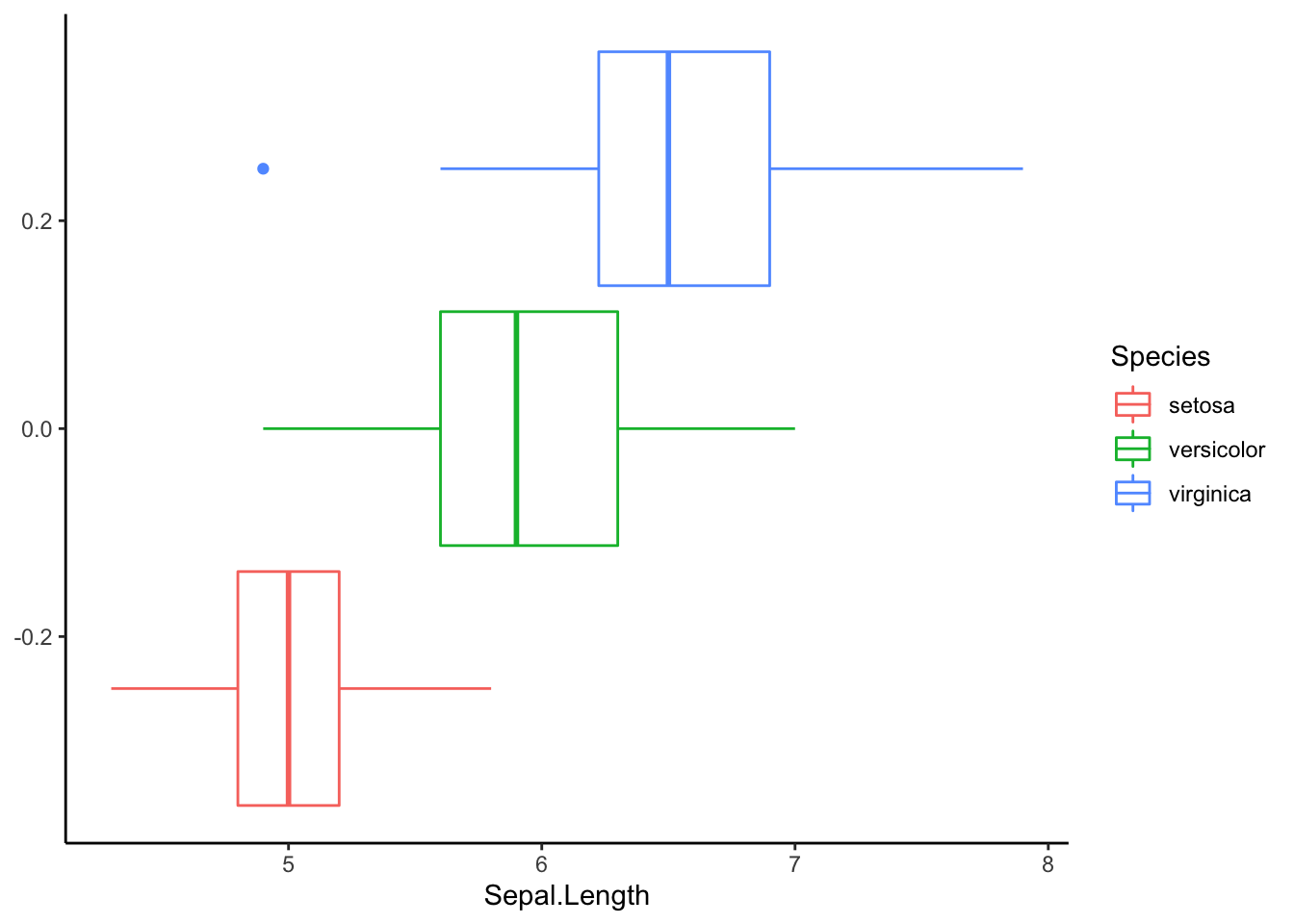
To run an ANOVA, we need to check if
- The variance is is equal for each group, and
- The data distributes normally within each group.
Let’s address the first point. Before doing a test, let us look at the figure above. The variance in each group looks relatively equal. Keep this in mind as we interpret Levene’s test for equal variances.
leveneTest(Sepal.Width ~ Species, data = iris)## Levene's Test for Homogeneity of Variance (center = median)
## Df F value Pr(>F)
## group 2 0.5902 0.5555
## 147What does the p-value suggest?
A p-value of 0.5555 suggested that the variances are not significantly different. With this assumption checked, we will proceed with ANOVA. Keep in mind we haven’t yet checked the normality. We will do it after running ANOVA.
We start by building an ANOVA model with the aov() function.
ANOVA. To run ANOVA in R, we need to pass two arguments to the aov() function. In general, this is what an ANOVA call looks like:
aov(y ~ x, data)For the
formulaparameter, the format isy ~ x, where the response variable (y) is to the left of the tilde (~), and the predictor variable (x) is to the right of the tilde.For the
dataparameter, we place the naame of the dataset we want to analyze.
In this example, we are asking if petal length is significantly different among the three species. We also need to tell R where to find the Sepal.Width and Species data, so we pass the variable name of the iris data.frame to the data parameter.
Let’s build the model:
Sepal.Width.aov <- aov(formula = Sepal.Width ~ Species, data = iris)Notice how when we execute this command, nothing printed in the console. This is because we instead sent the output of the aov call to a variable. If you just type the variable name, you will see the familiar output from the aov function:
Sepal.Width.aov## Call:
## aov(formula = Sepal.Width ~ Species, data = iris)
##
## Terms:
## Species Residuals
## Sum of Squares 11.34493 16.96200
## Deg. of Freedom 2 147
##
## Residual standard error: 0.3396877
## Estimated effects may be unbalancedTo see the results of the ANOVA, we call the summary() function:
summary(Sepal.Width.aov)## Df Sum Sq Mean Sq F value Pr(>F)
## Species 2 11.35 5.672 49.16 <2e-16 ***
## Residuals 147 16.96 0.115
## ---
## Signif. codes: 0 '***' 0.001 '**' 0.01 '*' 0.05 '.' 0.1 ' ' 1Answer to our question part 1: The species do have significantly different sepal width (P < 0.001).
However, ANOVA does not tell us which species are different. We can run a post hoc test to assess which species are different. A Tukey test comparing means would be one option. We will run the Tukey test after determining normality.
Now, let’s take a look at the normality. Once again, let’s visualize our data before running a test:
ggplot(iris, aes(Sepal.Length, fill=Species)) +
  geom_density(alpha=0.3) +
  theme_classic()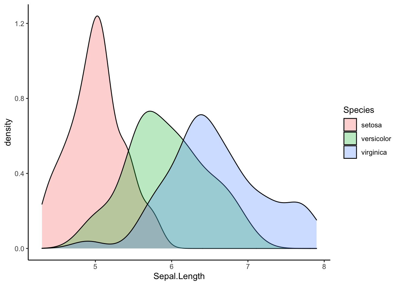
From the visualization alone, each species’ distribution of sepal lengths looks normal.
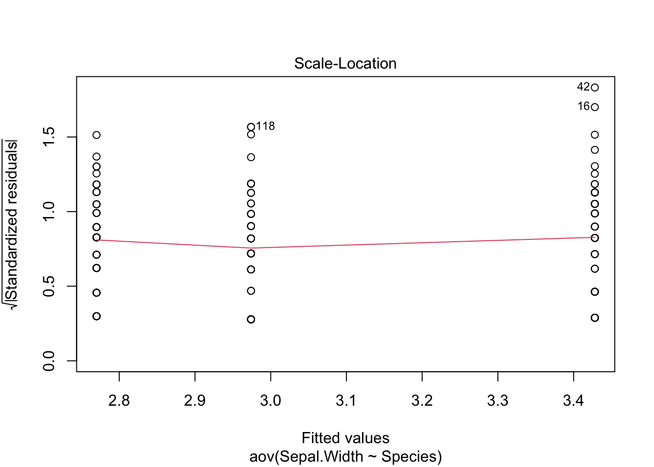
Now, we will plot the diagnostic figures.
plot(Sepal.Width.aov)
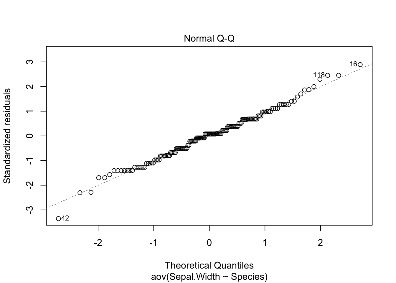
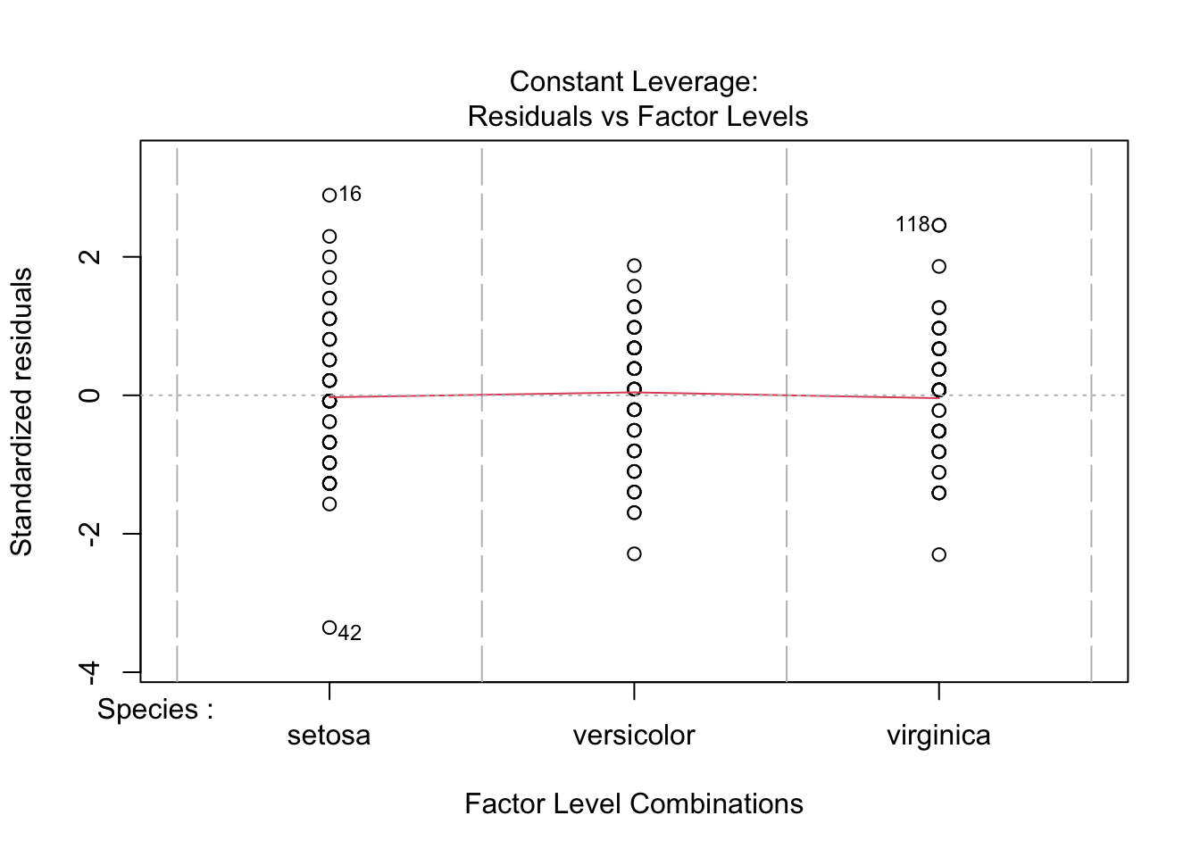
Most importantly, the residuals in Q-Q plot (upper right) should align with the line pretty well. If the residuals were to deviate from the line too much, the data would not be considered normal. If you still perform the ANOVA, you should view your results critically (or ignore them, at worst).
Recall that a residual is an “error” in result. More specifically, a residual is the difference of a given data point from the mean (\(x - \mu\)).
Please do not include diagnostic figures in the main text of your manuscripts. This might qualify for a supplementary figure at most.
Although we’ve also examined residuals with the Q-Q plot, we can also use a formal test:
residuals_Sepal_Width <- residuals(object = Sepal.Width.aov)
shapiro.test(x = residuals_Sepal_Width)
##
## Shapiro-Wilk normality test
##
## data: residuals_Sepal_Width
## W = 0.98948, p-value = 0.323A p-value of 0.323 suggested that the assumption of normality is reasonable.
So far, we have demonstrated
- Normality in distribution and
- Homogeneity in variance.
These two justified our choice for one-way ANOVA. The result of ANOVA also indicated that at least one species of the 3 has significantly different sepal width from others. Which ones are significantly different?
To do this, we need to run post-hoc test. Let’s do Tukey Honest Significant Differences (HSD) test. The nice thing is that TukeyHSD() can directly take the result of ANOVA as the argument.
TukeyHSD(Sepal.Width.aov)## Tukey multiple comparisons of means
## 95% family-wise confidence level
##
## Fit: aov(formula = Sepal.Width ~ Species, data = iris)
##
## $Species
## diff lwr upr p adj
## versicolor-setosa -0.658 -0.81885528 -0.4971447 0.0000000
## virginica-setosa -0.454 -0.61485528 -0.2931447 0.0000000
## virginica-versicolor 0.204 0.04314472 0.3648553 0.0087802Answer to our question part 2: The difference between every species of flower is significant at \(\alpha = 0.05\).
11.2.2 Non-parametric alternatives to ANOVA
In reality, your data usually will not fulfill every assumption for an ANOVA.
In case of a non-normal sample, there are two ways to address the problem:
- Apply appropriate data transformation techniques, or
- Use a non-parametric test.
I highly recommend you to explore data transformation. If you can rescue your data back to normal distribution, parametric tests usually allow you to do more powerful analysis. If you have exhausted your attempts to data transformation, you may then use non-parametric tests.
When your data doesn’t satisfy the normality or equal variance assumption, ANOVA is not the best test to use. The Kruskal-Wallis test doesn’t assume normality, but it does assume same distribution across groups (equal variance). If your data do not meet either assumption, you would want to use Welch’s one-way test. Now, let’s get back to gapminder data.
First, add another categorical variable calle Income_Level. This time we will split by the quartiles.
dat.1952 <- gapminder %>% filter(year == 1952)
border_1952 <- quantile(dat.1952$gdpPercap, c(.25, .50, .75))
dat.1952$Income_Level_1952 <- cut(dat.1952$gdpPercap,
                                  c(0, border_1952[1], border_1952[2], border_1952[3], Inf),
                                  c('Low', 'Low Middle', 'High Middle', 'High'))

dat.2007 <- gapminder %>% filter(year == 2007)
border_2007 <- quantile(dat.2007$gdpPercap, c(.25, .50, .75))
dat.2007$Income_Level_2007 <- cut(dat.2007$gdpPercap,
                                  c(0, border_2007[1],
                                    border_2007[2], border_2007[3], Inf),
                                  c('Low', 'Low Middle', 'High Middle', 'High'))
head(dat.1952)
## # A tibble: 6 × 7
## country continent year lifeExp pop gdpPercap Income_Level_1952
## <fct> <fct> <int> <dbl> <int> <dbl> <fct>
## 1 Afghanistan Asia 1952 28.8 8425333 779. Low
## 2 Albania Europe 1952 55.2 1282697 1601. Low Middle
## 3 Algeria Africa 1952 43.1 9279525 2449. High Middle
## 4 Angola Africa 1952 30.0 4232095 3521. High Middle
## 5 Argentina Americas 1952 62.5 17876956 5911. High
## 6 Australia Oceania 1952 69.1 8691212 10040. HighFor now, let’s focus on the data for the year 1952.
ggplot(data = dat.1952, aes(x = Income_Level_1952, y = lifeExp)) +
  geom_boxplot() +
  theme_classic()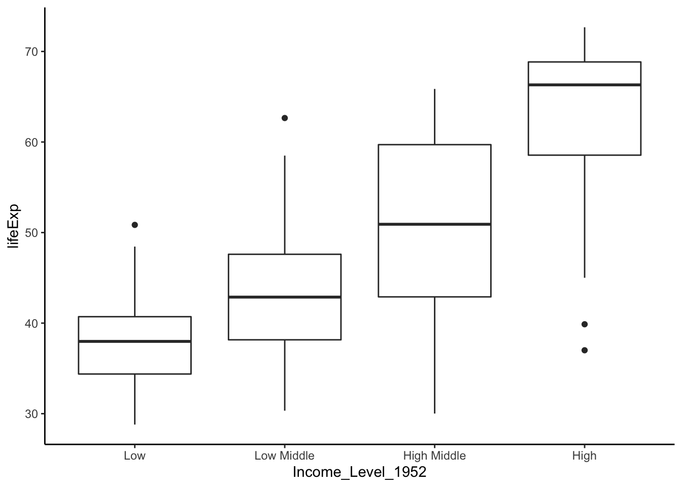
Let’s check the variance.
leveneTest(lifeExp ~ Income_Level_1952, data = dat.1952)## Levene's Test for Homogeneity of Variance (center = median)
## Df F value Pr(>F)
## group 3 4.3637 0.005714 **
## 138
## ---
## Signif. codes: 0 '***' 0.001 '**' 0.01 '*' 0.05 '.' 0.1 ' ' 1A p-value of 0.0047 suggested that the variances are significantly different. Therefore, we shoud not run ANOVA or Kruskal-Wallis. Let’s run Welch’s one-way test.
result <- oneway.test(lifeExp ~ Income_Level_1952, data = dat.1952)
result
##
## One-way analysis of means (not assuming equal variances)
##
## data: lifeExp and Income_Level_1952
## F = 69.799, num df = 3.000, denom df = 73.647, p-value < 2.2e-16What does the p-value mean?
A p-value of 2.2e-16 suggested that at least one category of Income_Level_1952 had values of lifeExp that are significantly different from others. Let’s run a post-hoc test to find out which categories are significant.
Since we are running a non-parametric test, an appropriate test would be Games-Howell post-hoc test. Unfortunately, R does not have a built-in function for Games-Howell. Let’s define a function to do this task.
Note: You don’t need to know how the code below works.
games.howell <- function(grp, obs) {
  # Create combinations
  combs <- combn(unique(grp), 2)

  # Statistics that will be used throughout the calculations:
  # n = sample size of each group
  # groups = number of groups in data
  # Mean = means of each group sample
  # std = variance of each group sample
  n <- tapply(obs, grp, length)
  groups <- length(tapply(obs, grp, length))
  Mean <- tapply(obs, grp, mean)
  std <- tapply(obs, grp, var)

  statistics <- lapply(1:ncol(combs), function(x) {
    mean.diff <- Mean[combs[2,x]] - Mean[combs[1,x]]
    # t-values
    t <- abs(Mean[combs[1,x]] - Mean[combs[2,x]]) / sqrt((std[combs[1,x]] / n[combs[1,x]]) + (std[combs[2,x]] / n[combs[2,x]]))
    # Degrees of Freedom
    df <- (std[combs[1,x]] / n[combs[1,x]] + std[combs[2,x]] / n[combs[2,x]])^2 / # numerator dof
      ((std[combs[1,x]] / n[combs[1,x]])^2 / (n[combs[1,x]] - 1) + # Part 1 of denominator dof
         (std[combs[2,x]] / n[combs[2,x]])^2 / (n[combs[2,x]] - 1)) # Part 2 of denominator dof
    # p-values
    p <- ptukey(t * sqrt(2), groups, df, lower.tail = FALSE)
    # sigma standard error
    se <- sqrt(0.5 * (std[combs[1,x]] / n[combs[1,x]] + std[combs[2,x]] / n[combs[2,x]]))
    # Upper Confidence Limit
    upper.conf <- lapply(1:ncol(combs), function(x) {
      mean.diff + qtukey(p = 0.95, nmeans = groups, df = df) * se
    })[[1]]
    # Lower Confidence Limit
    lower.conf <- lapply(1:ncol(combs), function(x) {
      mean.diff - qtukey(p = 0.95, nmeans = groups, df = df) * se
    })[[1]]
    # Group Combinations
    grp.comb <- paste(combs[1,x], ':', combs[2,x])
    # Collect all statistics into list
    stats <- list(grp.comb, mean.diff, se, t, df, p, upper.conf, lower.conf)
  })

  # Unlist statistics collected earlier
  stats.unlisted <- lapply(statistics, function(x) {
    unlist(x)
  })

  # Create dataframe from flattened list
  results <- data.frame(matrix(unlist(stats.unlisted), nrow = length(stats.unlisted), byrow=TRUE))
  # Select columns set as factors that should be numeric and change with as.numeric
  results[c(2, 3:ncol(results))] <- round(as.numeric(as.matrix(results[c(2, 3:ncol(results))])), digits = 3)
  # Rename data frame columns
  colnames(results) <- c('groups', 'Mean Difference', 'Standard Error', 't', 'df', 'p', 'upper limit', 'lower limit')
  return(results)
}
After defining the function, we can use it. If you decide to use the Games-Howell function, you can simply copy-and-paste it.
games.howell(grp = dat.1952$Income_Level_1952,  # groups, the categorical variable
             obs = dat.1952$lifeExp)            # observations, the continuous variable
## groups Mean Difference Standard Error t df p
## 1 Low : Low Middle 5.569 1.073 3.671 59.455 0.003
## 2 Low : High Middle 13.243 1.287 7.274 51.265 0.000
## 3 Low : High 24.536 1.247 13.917 53.954 0.000
## 4 Low Middle : High Middle 7.673 1.450 3.743 64.272 0.002
## 5 Low Middle : High 18.967 1.414 9.487 66.664 0.000
## 6 High Middle : High 11.294 1.583 5.046 68.787 0.000
## upper limit lower limit
## 1 9.580 1.559
## 2 18.077 8.408
## 3 29.210 19.863
## 4 13.081 2.266
## 5 24.235 13.699
## 6 17.187 5.401If you’re interested in learning more, check out this article on the Kruskal-Wallis test.
11.3 Beyond the one-way ANOVA
As seen in the previous example, a one-way ANOVA is a great tool for comparing multiple groups on one categorical variable such as income level. But what if we wanted to examine if life expectancy differs across the years 1952, 1972, and 2007 in addition to income level? In this case, we will need a two-way ANOVA.
Although we won’t cover a two-way ANOVA in this text, you can learn more about it in this article.