8 Central limit theorem

In this chapter, we will investigate the intuition behind the Central Limit Theorem (CLT). In short, the CLT states that if you have a bunch of samples and plotted the distribution of their means (not individual observations!), the distribution would look normal regardless of the population distribution. This theorem is incredibly powerful because it lets us to make inferences using statistical tests given a sufficient sample size.

8.1 Motivation

Imagine that we want to investigate whether Canadians recover faster than Americans from the common cold. How do we determine the probability that Canadians indeed recover faster than Americans?

The CLT helps us answer these questions by telling us that a “large enough” sampling distribution will follow a normal distribution. We can then use the properties of the normal distribution to compute the exact probability given our data.

8.2 CLT for means

Before formally exploring the CLT, play around with the CLT app! In short, the app takes samples from the “Population Distribution” and plots the mean of those samples in the “Sampling Distribution” histogram.

8.2.1 CLT Part 1

CLT Part 1. If our population is normal, our sampling distribution is also normal.

As always, let’s load the tidyverse.

library(tidyverse)

Many observed quantities follow normal distribution. Imagine that we have a population following normal distribution that has a mean of 10 and standard deviation of 2. If we draw samples from it, are we able to estimate its mean?

Note that rnorm() generates a vector of random numbers from a normal distribution.

(samp30 <- rnorm(n=30, mean=10, sd=2))

##  [1] 12.170742  8.903889  7.376290 13.060101 11.463640  8.849815 12.104130
##  [8] 13.629387 10.614798  9.385731  9.214561  9.296059 11.638205  8.769189
## [15] 13.139556  9.367540 10.943899  8.888327 11.693197  7.699428  8.063538
## [22] 10.237634  9.376883  8.504347  5.592137  9.195141  8.908910  9.634860
## [29] 10.138490  6.565606

mean(samp30)

## [1] 9.814201

Although the mean is not 10, it is pretty close. This should make sense; when we draw a sample to estimate the mean, we may get very close to the desired “true mean”, but we also expect some error. What if I repeat the estimation 1000 times with 30 samples?

# initializing our means vector
means10 <- as.vector(NA)

# taking 1000 samples
for (i in 1:1000) {
  samp10 <- rnorm(30, mean=10, sd=2)  # taking a sample with n=30
  means10[i] <- mean(samp10)          # recording sample mean
}

# plotting distribution of sample means
ggplot(as_tibble(means10), aes(value)) +
  geom_density(fill="#C5EBCB") +
  theme_classic()

What does this figure mean? Of the 1000 sample means we computed, most were very close to 10. The probability to overestimate and underestimate decreases as the estimation deviates from 10, our “true mean”. Further, the distribution of the sample means appears to follow a normal distribution.

8.2.2 CLT Part 2

CLT Part 2. Given a sufficient sample size, the sampling distribution of the means will look normal regardless of the original population distribution.

Notice that the CLT part 2 is a generalized version of the CLT part 1.

This time, let’s try sampling from a population that is uniformly distributed. For example, let’s create a population with 10,000 completely random numbers between 0 and 20:

uniform_popn <- runif(n=10000, min=0, max=20)  # our population distribution
ggplot(as_tibble(uniform_popn), aes(value)) +
  geom_density(fill="#C5EBCB") +
  theme_classic()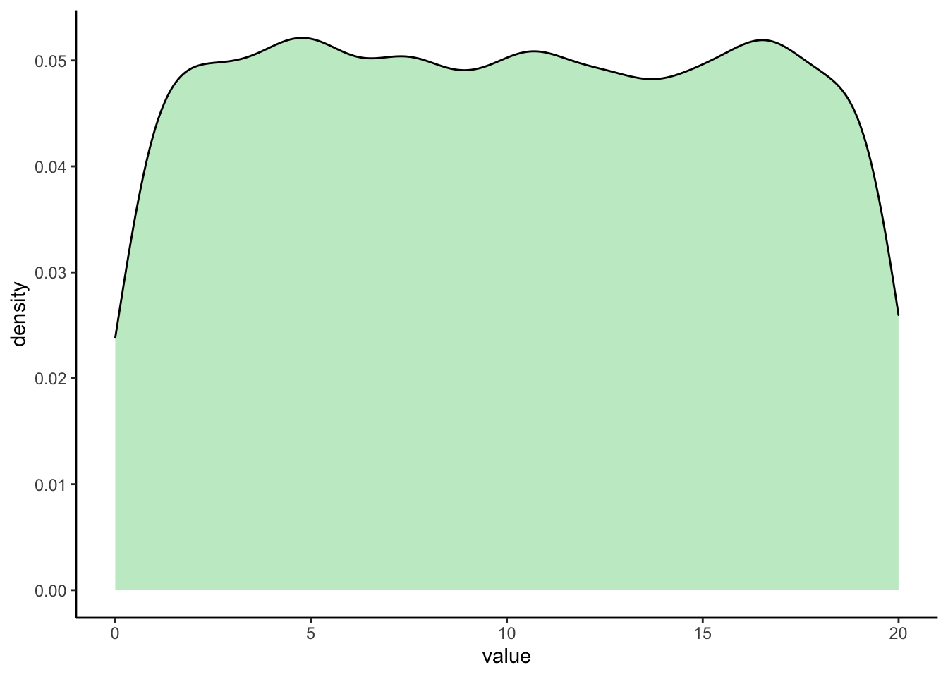

Now, we are going to repeatedly sample from uniform_popn and use the mean of that particular sample as our entry.

means10 <- as.vector(NA)
means100 <- as.vector(NA)
means1000 <- as.vector(NA)

# taking 1000 samples
for (i in 1:1000) {
  # each iteration, draw 10, 100, and 1000 samples from uniform_popn
  samp10 <- sample(uniform_popn, size = 10, replace = TRUE)
  samp100 <- sample(uniform_popn, size = 100, replace = TRUE)
  samp1000 <- sample(uniform_popn, size = 1000, replace = TRUE)
  # getting means of each sample
  means10[i] <- mean(samp10)
  means100[i] <- mean(samp100)
  means1000[i] <- mean(samp1000)
}

df <- rbind(
  data.frame(means = means10, sample_size = "10"),
  data.frame(means = means100, sample_size = "100"),
  data.frame(means = means1000, sample_size = "1000")
)

ggplot(df, aes(x = means, fill = sample_size)) + 
  geom_density(alpha = 0.3) +
  labs(x = "Sample means", y = "Density", fill = "Sample size") +
  theme_classic()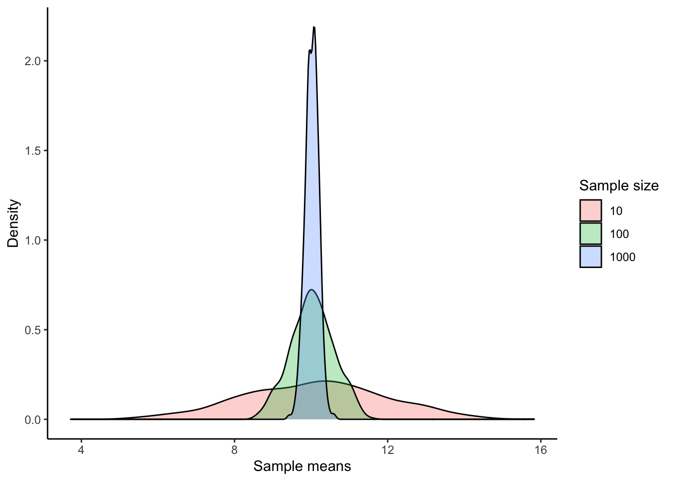

Notice two things:

With a larger sample size, your estimation for the mean will have a smaller variance.
Even though our original population was uniform (i.e., NOT normal), our sampling distribution looks normal. In fact, any population distribution will look normal given enough sample means.

As you can see, the bigger your sample size, the less variability there is, and the more the distribution looks like a normal distribution. More precisely, the bigger your sample size, the distribution of the sample means will be normally distributed, even if the population is not normally distributed. A good rule of “sufficiently large sample size” for means is n ≥ 30.

Pretty cool, right?

8.3 CLT for proportions

The CLT also holds for proportions.

Imagine we know the probability of not having the common cold is 0.9 and having the commmon cold is 0.1. Let’s record not having the common cold as 1 and having the common cold as 0. If I have a large enough sample size, we should expect the proportion to approach 0.9. Is this the case?

means100 <- as.vector(NA)
means1000 <- as.vector(NA)
means10000 <- as.vector(NA)

for (i in 1:10000) {
  sample100 <- sample(c(1, 0), prob = c(0.9, 0.1), replace = TRUE, size = 100)
  means100[i] <- mean(sample100)
  sample1000 <- sample(c(1, 0), prob = c(0.9, 0.1), replace = TRUE, size = 1000)
  means1000[i] <- mean(sample1000)
  sample10000 <- sample(c(1, 0), prob = c(0.9, 0.1), replace = TRUE, size = 10000)
  means10000[i] <- mean(sample10000)
}

df <- rbind(
  data.frame(means = means100, sample_size = "100"),
  data.frame(means = means1000, sample_size = "1000"),
  data.frame(means = means10000, sample_size = "10000")
)

ggplot(df, aes(x = means, fill = sample_size)) + 
  geom_density(alpha = 0.3) +
  labs(x = "Sample means", y = "Density", fill = "Sample size") +
  theme_classic()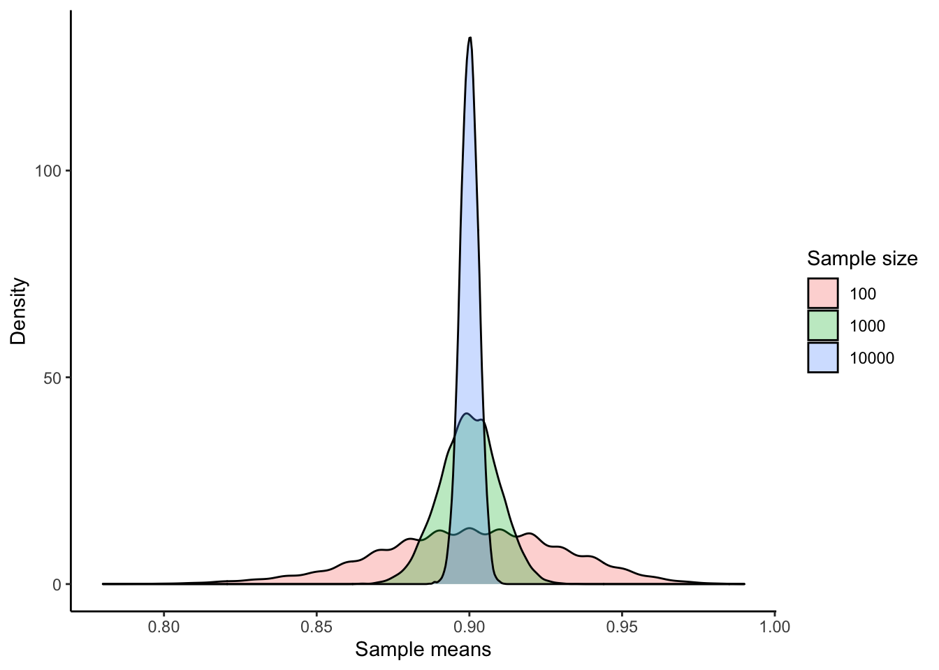

Can you explain the pattern that we observe with 100 samples? How about the height and width of other curves? What conclusions can we draw?

This example shows the power of the CLT—it allows us to predict a sampling distribution regardless of the original population.